Feature engineering

There are less than 15 unique variables in the provided data, around 70 features were created in order to finish with 85 before the modeling phase. I will describe interesting features below.

Machine learning

Since we are asked to predict which product will be reordered by customers, the product candidates for each customer is the list of product he has already bought atleast once. This can be seen as the binary classification problem where each tuple (user, product) is an observation targeted 0 or 1. I won’t explain in this post why this approach is more accurate and/or less computionnaly intensive than others (multi-label, Factorization machine, …) but focus on feature engineering.

Moreover, it was possible to predict that an user would reorder none of his past products. Predicting none is different from predicting a tuple (user, product). Therefore i created a second model for this purpose. Some features from this second model were extracted from the predictions of the first one.

Finals models are based on gradient boosted trees from LightGBM.

Workstation

I used to work locally (Macbook Pro, 2,9 GHz Intel Core i5, 16 Go Ram) on an sample of data in order to iterate quickly. My models were running but i had to wait one hour in order to submit my solution on all data.

During the last two weeks, i set up a virtual machine on Google Cloud with more CPU and RAM in order to get quickier results (and also be able to create new data based not only on the N orders but also the N-1 orders).

orders

Informations about orders :

• order_id
• user_id
• eval_set - If the order is part from train (last order from 125k users), test (last order from 75k users we need to predict on Kaggle), prior (past orders)
• order_number - First order is 1, last is N
• order_dow - Day of week
• order_hour_of_day
• days_since_prior_order - Number of days before the last order
• date - Inverse cumsum of days_since_prior_order (added for further FE)
• order_number_reverse - First order is N, last is 1 (added for further FE)
• last_basket_size - Number of products purchased in last order (added for further FE)

order_[prior|train|test]

• order_id
• user_id
• add_to_cart_order - Position of the product in the cart
• reordered - “Is the product reordered or not?”
• order_size - Size of the order (basket size)
• add_to_cart_order_inverted - Inverse position of the product in the cart (added for further FE)
• add_to_cart_order_relative - Relative position of the product in the cart (added for further FE)

products

Basic information about products, not much to add.

aisles

Basic information about aisles. Aisles contain products.

departments

Basic information about departements. Departements contain aisles.

users_products.f

Features based on the interaction of users and products :

• user_id
• product_id
• UP_order_strike - Detailed bellow
• up_nb_reordered - Number of times product was reordered
• up_last_order_number - Last order number (used for further FE)
• up_first_order_number - First order number (used for further FE)
• UP_date_strike - Detailed bellow
• up_add_to_cart_order_inverted_mean - Mean of add_to_cart_order_inverted - “Is the product added to the list at the end?”
• up_add_to_cart_order_mean - Mean add_to_cart_order -“Is the product added to the list in the beggining?”
• up_first_date_number - First date number (used for further FE)
• up_last_order_date - “When was the last (user,product) purchase”
• up_add_to_cart_order_relative_mean - “When is the product added to cart?”

UP_order_strike was my strongest feature in my model. Users reorder of does not products. So each series of (user, product) is a series of 0 and 1. Well it can be binary encoded, and allows to capture every pattern in a single feature and gives more importance to recent purchases (which is not the case with a basic mean).

Here is the Python code to help understanding how it is computed. I’ve choosen a power of 1/2 because i wanted “bigger is better” instead of “smaller is better”

order_prior["UP_order_strike"] = 1 / 2 ** (order_prior["order_number_reverse"])

users_products = order_prior. \
    groupby(["user_id", "product_id"]). \
    agg({..., \
         'UP_order_strike': {"UP_order_strike": "sum"}})

ie : For an user with 5 orders (NA means the product wasn’t bought yet)
0 0 0 0 1 = 1/2**5 = 0.03125 a product bought the first time and never purchased again
1 1 NA NA NA = 1/2**1 + 1/2**2 = 0.75 a product purchased the last two times
1 0 0 1 NA = 1/2**1 + 1/2**4 = 0.5625

Same idea is applied on date.

user_aisle_fe

Feature based on the interaction of users and aisles :

• user_id
• aisle_id
• UA_product_rt - Ratio of products purchased by the user in this aisle

user_department_fe

Feature based on the interaction of users and departments :

• user_id
• aisle_id
• UD_product_rt - Ratio of products purchased by the user in this department

users_fe

Feature engineering based on users :

• user_id
• U_rt_reordered - Reordering ratio - “does the user tends to purchase new products?”
• U_basket_sum - Number of products purchased
• U_basket_mean - Mean number of products purchased per order (basket size) - “how much products does the user buys?”
• U_basket_std - Standard deviation number of products per order - “does the user have different basked size?
• u_reorder_rt_bool - Mean of “the product was reordered atleast once”
• u_active_p - Number of unique products
• U_date_inscription - Date of the first order
• U_days_since_std - Standard deviation of days since prior order - “does the user have different days_since_prior_order?
• U_days_since_mean - Mean of days since prior order - “does the user orders often or not?”
• U_none_reordered_mean - Mean of “no products were reordered, only new products”
• U_none_reordered_strike - Binary encoding (explained in detail in user_product part above) of “no products were reordered, only new products”

products_fe_mod

Feature engineering on products :

• product_id
• P_recency_order_r - Mean(order_number_reverse)
• P_recency_order - Mean(order_number)
• p_add_to_cart_order - Mean(add_to_cart_order)
• p_count - Number of time the product was bought
• p_reorder_rt - Mean of the users’ mean of reaorder ratio of the product
• P_recency_date - Mean(date)
• p_reorder_rt_bool - Mean of the users’ “the product was reordered at least once”
• p_active_user - Number of unique users who purchased the product atleast once
• p_size - Number of time the product was reordered
• p_trend_rt - Number of times the product was bought in order N / number of times the product was bought in order N-1
• p_trend_diff - Number of times the product was bought in order N minus number of times the product was bought in order N-1
• p_freq_order - Mean number of orders before the product is reordered
• p_freq_days - Mean days before the product is reordered
• user_fold - user folder - i created the above stastitics for each user folder, i did it because i wanted to include data from training data and while avoiding data leak (in order to consolidate the products statistics), but in the end it didn’t help much

aisles_fe

Feature engineering on aisles :

• aisle_id
• a_reorder_rt - Mean of the users’ mean of reaorder ratio in aisle
• a_count - Number of time a product was bought in the aisle
• a_add_to_cart_order - Mean add_to_cart_order of the products bought in the aisle
• a_reorder_rt_bool - Mean of the users’ “the product was reordered at least once” in this aisle
• a_active_user - Number of unique users in the aisle

departments_fe.f

Basicly the same feature engineering that on aisles but on departments :

• department_id
• d_reorder_rt - Mean of the users’ mean of reaorder ratio in department
• d_count - Number of time a product was bought in the department
• d_add_to_cart_order - Mean add_to_cart_order of the products bought in the department
• d_reorder_rt_bool - Mean of the users’ “the product was reordered at least once” in this department
• d_active_user - Number of unique users in the department

product2vec.f

Features created from product embeddings. It’s the same idea as word embedding but on products. Each orders is considered as a sentence. Products can be seen as words.

Find out more here. The idea was nice but in the end it didn’t help much and even not at all. But it did cost computing power.

mult_none_cv

Features calculed from the first stage model’s predictions :

• order_id
• user_id
• pred_none_prod - \(\prod_{i=1}^{N} 1-p_{i,u}\) with \(p_{i,u}\) the probability of reordering for product i, user u from the first model - probability of reordering None if there were independance betweens products (which is not the case, that’s why a 2nd model is needed)
• pred_basket_sum - \(\sum_{i=1}^{N} 1-p_{i,u}\) with \(p_{i,u}\) the probability of reordering for product i, user u from the first model - estimated basket size of reordered products
• pred_basket_std - standard deviation of \(p_{i,u}\) for all products i of the user u

It is done with cross-validation in order to avoid any data leak.

Additionnal features

Once i joined every tables from my feature engineering store, i computed some simple additionnal features based on feature from different tables :

• user_id
• product_id
• UP_rt_reordered - Reordering ratio of the product
• UP_rt_reordered_since_first - Reordering ration of the product since the first time product was bought
• UP_days_no-reordered - Number of days since the product wasn’t bought
• UP_freq_nb_no-reordered - UP_days_no-reordered divided by up_add_to_cart_order_mean - should be able to capture periodicity
• UP_sum_basket_rt - up_nb_reordered divided by U_basket_sum
• O_days_since_prior_order_diff - days_since_prior_order minus days_since_prior_order_mean
• O_days_since_prior_order_rt - days_since_prior_order divided days_since_prior_order_mean

Target - user_past_product

Table created in order to list products reordered in train (positive sample) and all products ordered atleast once but not reordered in train set (negative sample).

• user_id
• product_id
• reordered - Our target - “Was the product reordered in the train set?”

Note : For the test set, a list of (user,product) candidate was generated.

Models

Well i don’t want to focus on this part, morevore there is nothing amazing. I did a simple 90% train / 10% validation split based on users for both models.

Here are the parameters for the first model :

lgb_train = lgb.Dataset(X_train, label=y_train)
param = {'objective': 'binary', 
          'metric': ['binary_logloss'], 
          'learning_rate':0.025, 
          'verbose': 0}

And the second one (predicting None) :

lgb_train_none = lgb.Dataset(X_train_none, label=y_train_none, max_bin=100)
param_none = {'objective': 'binary', 
              'metric': ['binary_logloss'], 
              'learning_rate':0.05,
              'num_leaves':3, 
              'min_data_in_leaf':500, 
              'verbose': 0}

Features importance

Bellow the features importance from both models. It highlights how important are each features we created.

I’m not good at plotting on Python, and i’ve some difficulties with lightgbm plotting API, therefore sorry for the imperfects graphics.

First model (only top40 otherwise it is not lisible anymore) :

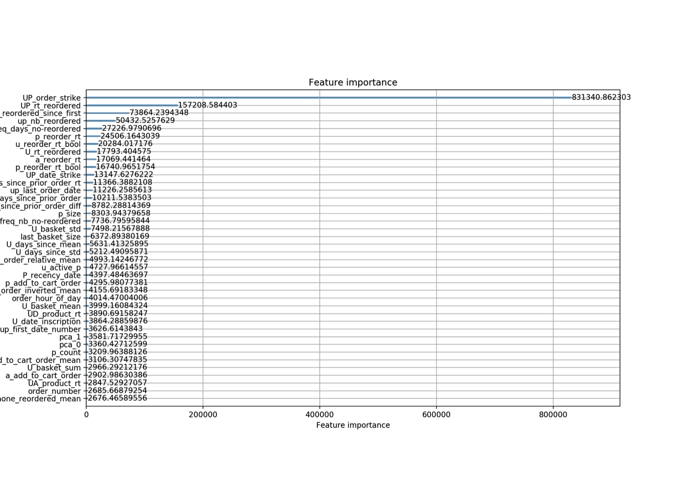
We can clearly see that UP_order_strike the binary encoding based claim the first place.

Second model :

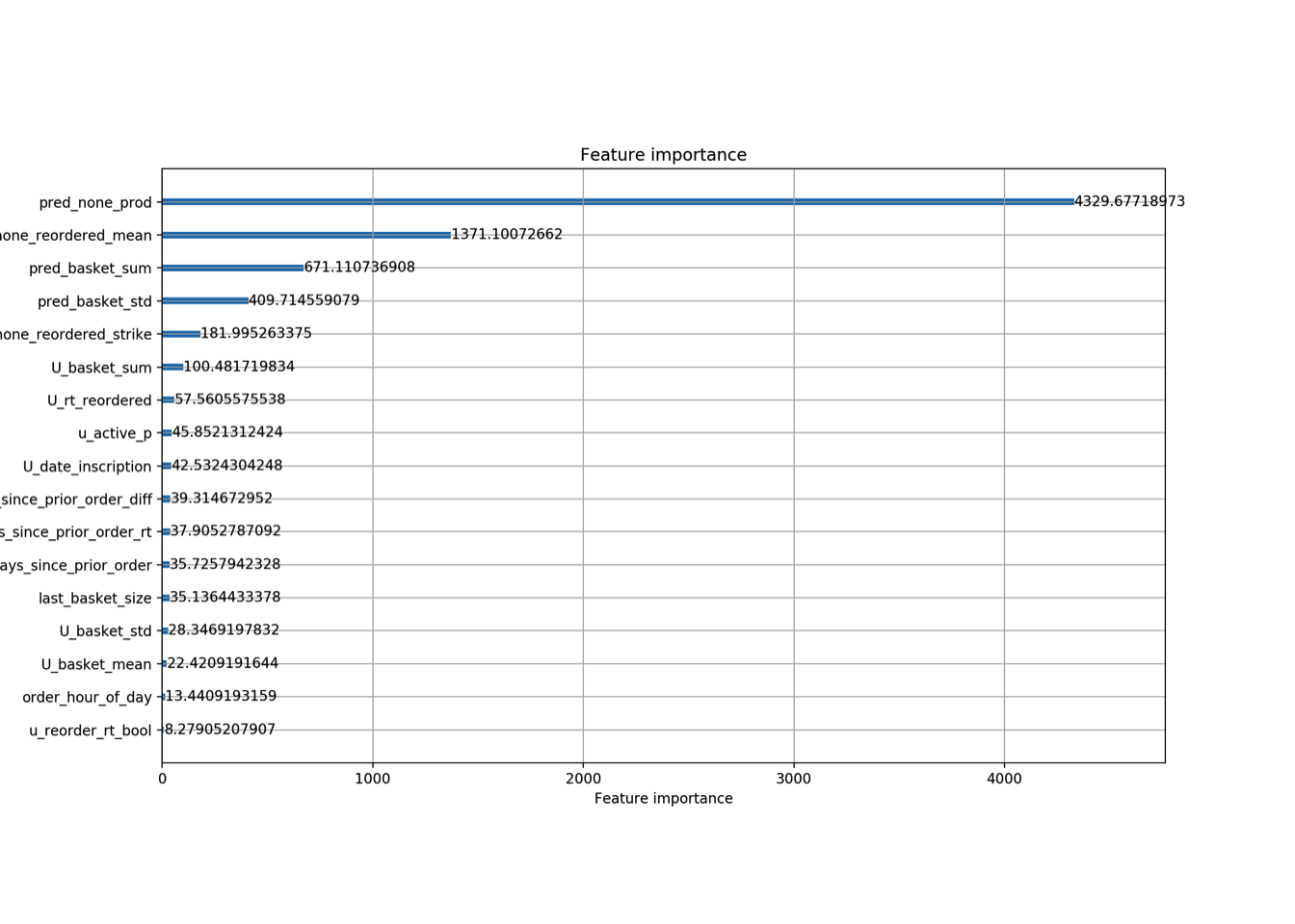
The features extrated from first models prediction are placed high (top4).